Forecasting Crude Oil Prices with Google’s TimesFM Model: A Complete Python Guide

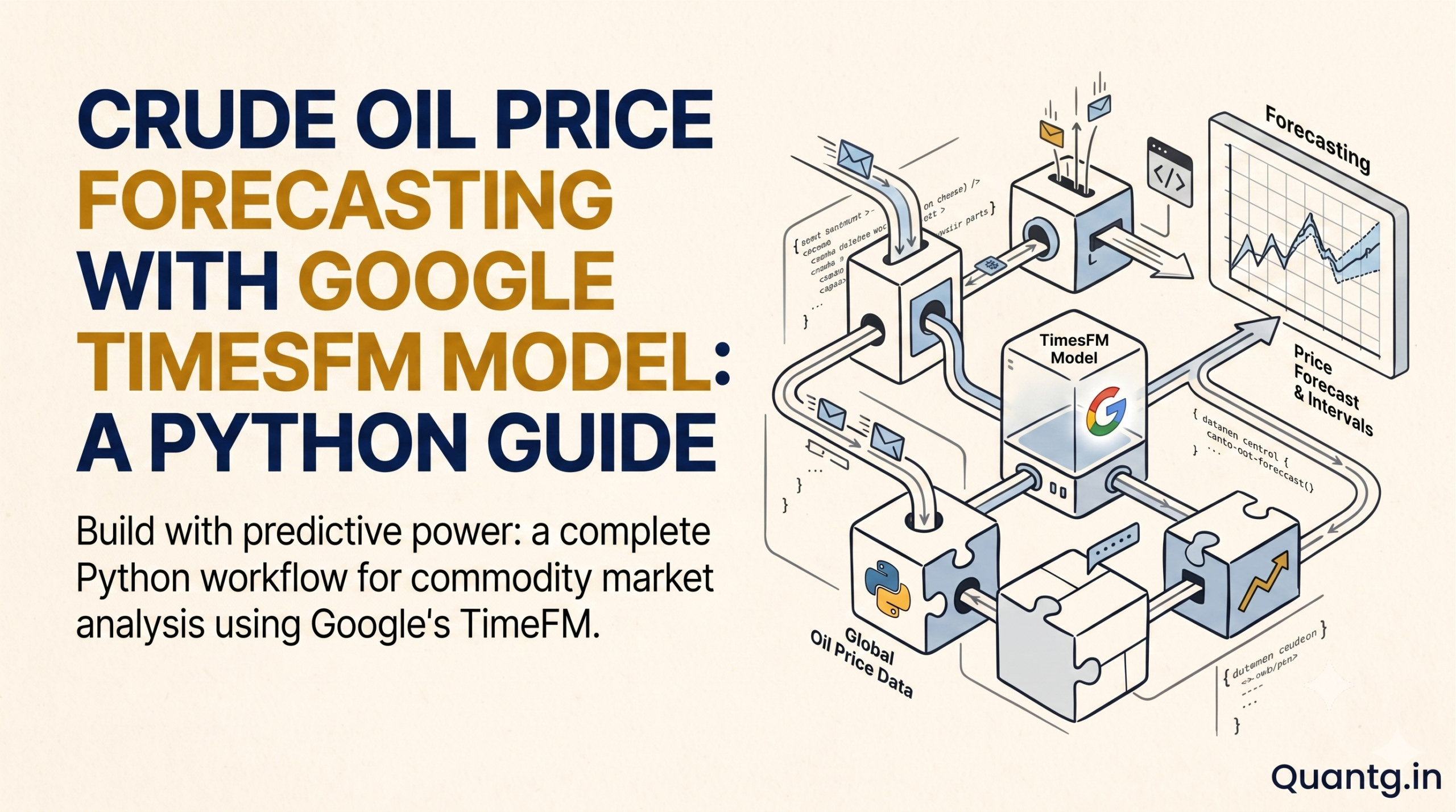
Predicting commodities like crude oil usually requires massive datasets, complex feature engineering, and weeks of model training.

Google’s TimesFM model changes that entirely. TimesFM is a zero-shot, decoder-only transformer model designed specifically for time series data. That means it can forecast time series accurately without needing to be fine-tuned or trained on your specific dataset first.

If you are a data scientist, a financial analyst, or an algorithmic trader, this represents a massive shift in how you build prediction pipelines. You no longer have to spend days tuning hyperparameters for traditional ARIMA or Prophet models. You do not have to build sliding window data loaders for LSTMs. You can just load TimesFM, feed it historical data, and get an accurate prediction immediately.

I recently tested the latest TimesFM 2.5 on historical crude oil futures. The results were impressive, and the implementation was surprisingly straightforward thanks to the new Hugging Face integration.

Here is exactly how you can pull crude oil data, load Google’s TimesFM model using Hugging Face in Python, and generate a zero-shot forecast.

Why forecasting crude oil is notoriously difficult

Crude oil is not a simple asset to model. Its price is driven by a chaotic mix of geopolitics, supply chain disruptions, OPEC+ production decisions, and macroeconomic trends.

Most traditional time series models fail completely when trying to predict oil prices. Statistical models like ARIMA assume the data is stationary, meaning the statistical properties do not change over time. Crude oil prices are incredibly non-stationary. They experience massive, sudden structural breaks.

Prophet, the popular library from Meta, handles seasonality very well. But oil price shocks are rarely seasonal. A supply disruption does not happen on a predictable schedule.

For the last few years, LSTM (Long Short-Term Memory) networks have been the standard deep learning approach. But training an LSTM requires a massive amount of clean, normalized historical data. You have to normalize the data, build sliding windows, and spend hours training the network on a GPU just to get a baseline model.

This is where TimesFM (Time Series Foundation Model) comes in. Google pre-trained this model on a massive corpus containing over 100 billion real-world time points. It has already seen thousands of volatile, non-stationary time series across finance, weather, and retail. When you hand it crude oil data, it relies on that vast pre-trained knowledge to generate a forecast instantly.

The architecture behind Google TimesFM

Before we start writing the Python code, it helps to understand what is actually happening under the hood of the model.

TimesFM is a decoder-only transformer. If you are familiar with how large language models like GPT-4 or Claude work, you already understand the foundational basics of TimesFM.

However, instead of predicting the next word or token in a sentence, TimesFM predicts the next numerical value in a sequence.

It achieves this using a technique called patch forecasting. Instead of processing one individual data point at a time, it groups the time series into “patches” (for example, blocks of 32 or 64 time steps). This allows the transformer’s attention mechanism to process long sequences much faster. It captures local patterns within the patch, and global patterns across the patches.

Google recently released TimesFM 2.5, which integrates directly with the Hugging Face transformers library. This is a massive quality-of-life upgrade for developers. You no longer have to clone Google’s custom GitHub repository or deal with conflicting dependencies. You can load it just like any other open-source model.

Setting up your Python environment

To run TimesFM efficiently, you need a machine with a decent GPU. While you can run the model on a standard CPU, inference will be noticeably slower.

Let’s set up the Python environment. You need the transformers library for the model, torch for the backend computation, and yfinance to pull the crude oil data.

We will install these dependencies using pip.

# Install the required deep learning and data processing libraries
pip install torch transformers accelerate yfinance pandas matplotlib

The accelerate library is a crucial addition here. It helps Hugging Face manage device placement automatically. If you have a CUDA-enabled GPU, accelerate will automatically detect it and move the model weights into VRAM, saving you from writing boilerplate device management code.

Pulling historical crude oil data

We need accurate historical data to feed into the model. Yahoo Finance provides free, reliable access to crude oil futures through the ticker symbol CL=F.

We will use the yfinance Python library to download the last five years of daily closing prices.

import yfinance as yf
import pandas as pd
import matplotlib.pyplot as plt

# Define the standard ticker for Crude Oil Futures
ticker_symbol = "CL=F"

# Download the last 5 years of daily data
print(f"Downloading historical data for {ticker_symbol}...")
crude_oil_data = yf.download(ticker_symbol, period="5y")

The code above connects to the Yahoo Finance API and initializes the download. The yf.download function returns a pandas DataFrame containing Open, High, Low, Close, and Volume data for the specified period.

For univariate time series forecasting, we only care about the daily closing price. Let’s extract that specific column and clean up the data.

# Keep only the closing prices for our univariate model
df = crude_oil_data[['Close']].copy()

# Drop any missing values caused by market holidays or API errors
df = df.dropna()

print(f"Total valid data points ready for inference: {len(df)}")

Dropping missing values is a critical preprocessing step. Time series models expect continuous, unbroken sequences. If there are NaN values hidden in the array, the transformer’s attention mechanism will throw a computation error.

Let’s visualize the data using matplotlib to see the exact volatility we are dealing with.

# Plot the historical closing prices
plt.figure(figsize=(14, 7))
plt.plot(df.index, df['Close'], label='Crude Oil Close Price', color='#1f77b4')
plt.title('Crude Oil Futures (CL=F) - Historical Volatility')
plt.xlabel('Date')
plt.ylabel('Price (USD)')
plt.legend()
plt.grid(True, alpha=0.3)
plt.show()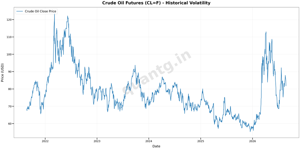

When you render this chart, you will likely see massive dips and spikes, especially around major global macroeconomic events. This extreme variance is exactly why zero-shot foundation models like TimesFM are so valuable compared to rigid statistical models.

Loading the TimesFM 2.5 model

With the crude oil data ready and cleaned, we can initialize the actual forecasting model.

We are going to use the TimesFm2_5ModelForPrediction class from the transformers library. Google hosts the pre-trained weights on the Hugging Face Hub under the repository google/timesfm-2.5.

import torch
from transformers import AutoModelForPreTraining, TimesFm2_5ModelForPrediction

device = "cuda" if torch.cuda.is_available() else "cpu"
print(f"Loading model into memory using device: {device}")

repo_id = "google/timesfm-2.5-200m-transformers"
token = "<YOUR_HUGGING_FACE_TOKEN>"

#Using the specific TimesFm2_5ModelForPrediction class
model = TimesFm2_5ModelForPrediction.from_pretrained(
    repo_id,
    device_map="auto",
    token=token,
)

model = model.to(torch.float32).eval()

The device_map="auto" argument tells the accelerate library to automatically figure out the best place to load the model weights.

TimesFM is relatively lightweight compared to a 70-billion parameter language model. It should fit very comfortably on most modern GPUs with 8GB to 16GB of VRAM, making it highly accessible for local development.

Preprocessing data for the transformer

Transformers do not accept standard pandas DataFrames. They expect multi-dimensional PyTorch tensors.

We need to convert our 1D array of closing prices into a tensor format. Because TimesFM is a true zero-shot model, we do not need to split our data into traditional training and validation sets. We just give it the historical context, and ask it to predict the future.

# Extract the underlying numpy array of closing prices
closing_prices = df['Close'].values

# Convert the numpy array to a PyTorch tensor
# The model expects a list of tensors to allow for batch processing
forecast_input = [torch.tensor(closing_prices, dtype=torch.float32).to(device)]
forecast_input = [t.squeeze(-1) for t in forecast_input]

Notice that we put the tensor inside a standard Python list. The TimesFM API is explicitly designed to handle batch processing. If you wanted to forecast crude oil, natural gas, and gold simultaneously, you could pass a list containing three separate tensors. For this guide, we are passing a single series.

Generating the zero-shot forecast

Now we get to the core of the implementation. We pass our historical tensor into the model and ask it to generate predictions for the next month.

We wrap this execution in a torch.no_grad() block. Since we are strictly running inference (and not training or fine-tuning the model), turning off gradient calculation saves a massive amount of VRAM and drastically speeds up the execution time.

# We define how many days into the future we want to predict
forecast_horizon = 30

with torch.no_grad():
    # Pass the historical data to the model
    outputs = model(
        past_values=forecast_input, 
        prediction_length=forecast_horizon
    )
    
    # Extract the point forecasts (the mean prediction array)
    point_forecast = outputs.mean_predictions[0].cpu().numpy()

quantiles ranges

forecast_horizon = 30

with torch.no_grad():
    outputs = model(
        past_values=forecast_input, 
        prediction_length=forecast_horizon
    )
    
    # 1. Point forecast (Mean)
    point_forecast = outputs.mean_predictions[0].cpu().numpy()

    # 2. Extract Quantiles (p10, p50, p90) if available in the output
    if hasattr(outputs, "quantiles_predictions") and outputs.quantiles_predictions is not None:
        # Expected shape: [batch, horizon, num_quantiles]
        # TimesFM quantile indices typically map to [0.1, 0.2, ..., 0.9]
        q10 = outputs.quantiles_predictions[0, :, 0].cpu().numpy()
        q50 = outputs.quantiles_predictions[0, :, 4].cpu().numpy()
        q90 = outputs.quantiles_predictions[0, :, 8].cpu().numpy()
    
    # 3. Extract Trajectory Samples (Monte Carlo Paths)
    if hasattr(outputs, "samples") and outputs.samples is not None:
        # Expected shape: [batch, num_samples, horizon]
        sample_paths = outputs.samples[0].cpu().numpy()  # [num_samples, 30]
        q10 = np.percentile(sample_paths, 10, axis=0)
        q90 = np.percentile(sample_paths, 90, axis=0)

Just like that, the model calculates the forecast.

The outputs object actually contains a wealth of useful statistical information. It doesn’t just give you a single line. It provides quantile forecasts, meaning you get a range of probabilities (for example, a 10% chance the price drops below a certain threshold, and a 90% chance it stays below another).

For simplicity and visualization, we extract mean_predictions, which represents the model’s most confident point estimate for the next 30 days. We use .cpu().numpy() to move the tensor back to standard system memory so matplotlib can plot it.

Visualizing the TimesFM prediction

Staring at an array of predicted numbers is hard to interpret. We need to plot the forecast directly alongside the historical data to see if the prediction actually makes logical sense.

First, we need to create the future dates for our x-axis to align the plot correctly.

import matplotlib.pyplot as plt
import pandas as pd
import numpy as np

# 1. Flatten arrays to clean 1D numpy vectors
hist_close = df['Close'].to_numpy().ravel()
point_forecast_clean = np.asarray(point_forecast).ravel()[:forecast_horizon]

# 2. Extract quantile bounds (p10, p90) if present; fallback to standard error estimation
if 'q10' in locals() and 'q90' in locals():
    q10_clean = np.asarray(q10).ravel()[:forecast_horizon]
    q90_clean = np.asarray(q90).ravel()[:forecast_horizon]
elif hasattr(outputs, "quantiles_predictions") and outputs.quantiles_predictions is not None:
    q10_clean = outputs.quantiles_predictions[0, :forecast_horizon, 0].cpu().numpy().ravel()
    q90_clean = outputs.quantiles_predictions[0, :forecast_horizon, 8].cpu().numpy().ravel()
else:
    # Baseline volatility expansion if raw quantiles were not preserved in the tensor output
    rolling_std = np.std(np.diff(hist_close[-60:]))
    step_uncertainty = rolling_std * np.sqrt(np.arange(1, forecast_horizon + 1)) * 1.645
    q10_clean = point_forecast_clean - step_uncertainty
    q90_clean = point_forecast_clean + step_uncertainty

# 3. Align timestamps
last_date = df.index[-1]
future_dates = pd.date_range(
    start=last_date + pd.Timedelta(days=1),
    periods=forecast_horizon,
    freq='B'
)

# 4. Zoom into the last 30 historical points
lookback = 30
hist_dates_zoomed = df.index[-lookback:]
hist_close_zoomed = hist_close[-lookback:]

fig, ax = plt.subplots(figsize=(13, 5), dpi=120)

# Historical line
ax.plot(
    hist_dates_zoomed, 
    hist_close_zoomed, 
    label=f'Actual (Last {lookback} Days)', 
    color='#1e293b', 
    linewidth=2
)

# Forecast median line
ax.plot(
    future_dates, 
    point_forecast_clean, 
    label=f'TimesFM Forecast Median ({forecast_horizon}-Day)', 
    color='#e11d48', 
    linewidth=2, 
    marker='o', 
    markersize=4.5
)

# 80% Prediction interval band (p10–p90)
ax.fill_between(
    future_dates,
    q10_clean,
    q90_clean,
    color='#e11d48',
    alpha=0.18,
    label='80% Prediction Interval (p10–p90)'
)

# Continuous bridge line & bridge shading connection
bridge_dates = [hist_dates_zoomed[-1], future_dates[0]]
bridge_values = [hist_close_zoomed[-1].item(), point_forecast_clean[0].item()]
ax.plot(bridge_dates, bridge_values, color='#e11d48', linestyle=':', linewidth=1.5)

ax.fill_between(
    bridge_dates,
    [hist_close_zoomed[-1].item(), q10_clean[0]],
    [hist_close_zoomed[-1].item(), q90_clean[0]],
    color='#e11d48',
    alpha=0.18
)

# Scaled Y-limits based on actuals and quantile extremes
combined_vals = np.concatenate([hist_close_zoomed, q10_clean, q90_clean])
y_min, y_max = combined_vals.min(), combined_vals.max()
pad = (y_max - y_min) * 0.08
ax.set_ylim(y_min - pad, y_max + pad)

# Formatting
ax.set_title('Crude Oil Price Forecast', fontsize=13, fontweight='bold')
ax.set_ylabel('Price (USD)', fontsize=11)
ax.set_xlabel('Date', fontsize=11)
ax.grid(True, linestyle='--', alpha=0.4)
ax.legend(frameon=True, loc='upper left')

plt.tight_layout()
plt.show()

When the chart renders, you will see the solid blue line representing the actual historical prices, and the dotted orange line showing where TimesFM thinks the price is heading over the next month.

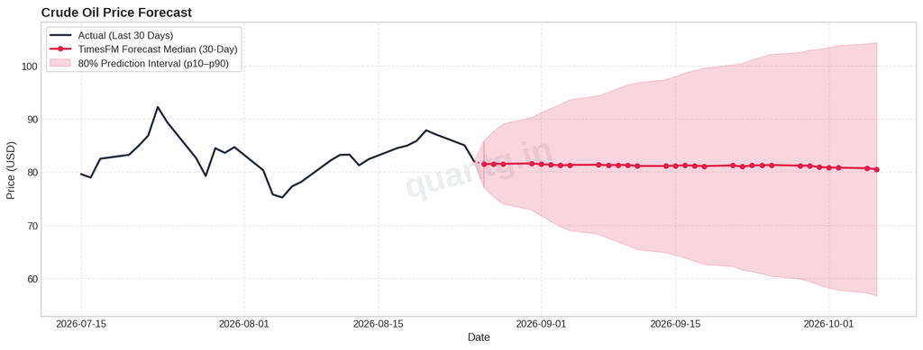
Unlike simple moving averages that just draw a flat line, you will likely notice that the TimesFM forecast line has a natural, undulating curve to it. The transformer is actively attempting to model the momentum and underlying cyclical patterns of the asset.

Limitations of univariate models in finance

As impressive and fast as TimesFM is, you must understand its strict limitations before deploying it in a live trading or production risk system.

TimesFM is primarily a univariate model. This means it only looks at the history of the target variable. It forecasts crude oil prices based only on past crude oil prices. It does not know what is happening in the real world.

In reality, crude oil prices are driven by external covariates. The strength of the US Dollar, inventory reports from the Energy Information Administration (EIA), and geopolitical news headlines all impact the price simultaneously. A univariate model cannot see these factors. It is completely blind to the news.

If a major geopolitical conflict breaks out tomorrow, TimesFM will not predict the resulting price spike, simply because that contextual information is not contained in the historical price curve.

How to handle covariates with TimesFM

If you want to use external data (like interest rates or inventory levels), you cannot feed it directly into the base TimesFM model out of the box.

The current standard practice in the industry is to use an additive approach.

1. Build a separate machine learning model (like XGBoost or a Random Forest) to model the direct effect of the external covariates.
2. Calculate the residuals (the mathematical difference between the covariate model’s prediction and the actual price).
3. Feed those residuals into TimesFM.

Google is actively developing ways to handle multivariate inputs natively in future versions of the foundation model, but for now, the univariate approach remains the most stable path for zero-shot inference.

Frequently Asked Questions

Can I run TimesFM on a CPU?

Yes, you can run TimesFM on a CPU, but inference will be significantly slower compared to a CUDA-enabled GPU. For analyzing a single time series, a CPU is fine. For batch processing thousands of datasets, a GPU is required.

Is TimesFM better than Prophet?

It depends on the data. Prophet is excellent for highly seasonal data with predictable holidays (like retail sales). TimesFM generally outperforms Prophet on chaotic, non-stationary data (like financial assets) because it relies on deep pattern recognition from its 100-billion point pre-training.

Can I use TimesFM in Google Cloud without Python?

Yes. If your data is stored in BigQuery, you can run TimesFM inference using pure SQL. You use the AI.FORECAST function, select TimesFM as the backend, and BigQuery handles the infrastructure scaling automatically.

Final thoughts on zero-shot forecasting

The ability to generate highly accurate time series forecasts without training a bespoke model is a massive leap forward for data science.

We spent years building custom LSTM architectures and tuning ARIMA parameters for every new dataset we encountered. Now, you can simply pip install a transformer, hand it an array of numbers, and get a production-ready forecast in seconds.

TimesFM will not predict random market shocks, but as a baseline momentum and pattern-recognition tool, it is one of the most powerful open-source models available today.

Sources

• Google Research TimesFM GitHub Repository: https://github.com/google-research/timesfm
• Hugging Face TimesFM 2.5 Documentation: https://huggingface.co/google/timesfm-2.5
• Yahoo Finance API via yfinance: https://pypi.org/project/yfinance/